Neo Quest: Blockchain Powered AI Art Competition

In 2022 at the very beginning of the whole AI buzz(that started with AI image generators) when artists were thinking AI is going to take their job, I worked on an interesting project for an AI art competition concept where participants compete to recreate a target image using only AI prompts. The idea was simple:

If you think it's easy, buy a ticket and join the competition.

The goal was to show artists it's not that easy to recreate what's in your mind only using your words. Well NOW it's 2025 and thats not valid anymore, but in my defense, back then we only had Stable Diffusion and early version of Midjourney which you could only use via Discord, and the quality wasn't that good. Here is the very first image i generated using Midjourney:

The platform had daily competitions, and it was based on Blockchain (so everything was transparent and safe) and users needed to buy a ticket, and had 1 hour and 100 prompts to recreate the target image. The winner is determined by whose generated image is most similar to the target and the prize was the 80% of the collected tickets. In this post I will share how I approached the image similarity scoring system (The blockchain part wasn't that big of a deal to explain)

‍

‍

The Problem:

The core challenge was simple: given one target image per competition, how do you accurately rank candidate submissions? This might sound straightforward at first, but as I dug deeper, I realized the classical approaches I had used before were fundamentally flawed for this task.

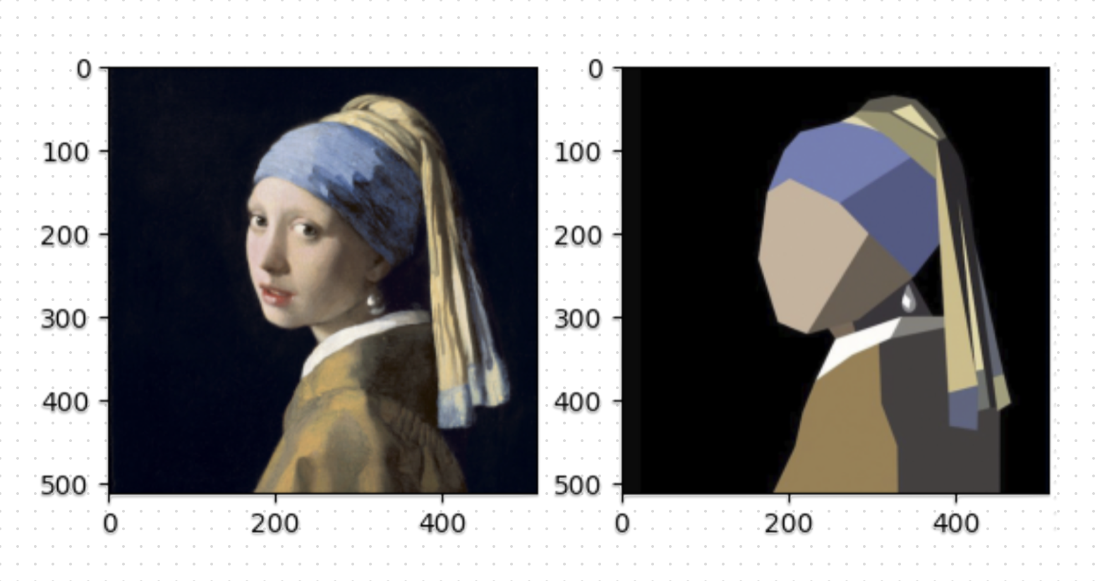
I chose the Girl with Pearl Earring as the target image, and found different meme versions of it online to use as the attempts to test the system

‍

How I Did It initially (Classic Image Processing)

In my first attempts at image comparison, I threw everything at the problem. I combined dozens of hand-crafted metrics from different libraries and image processing techniques. The idea was to calculate all these metrics between the target and candidate images, normalize them somehow, and combine them with some weights to produce a final similarity score. I will try to briefly explain the methods I have tried and show the results for these two images:

‍

‍

Global Histogram Comparisons and Pixel Statistics

This method compares the overall color or intensity distribution of two images by analyzing their histograms and basic pixel statistics, providing a simple measure of similarity. It has two sides:

• Histogram Difference: Compares color or intensity histograms

• Flattened Correlation: Correlation of flattened grayscale pixel arrays.

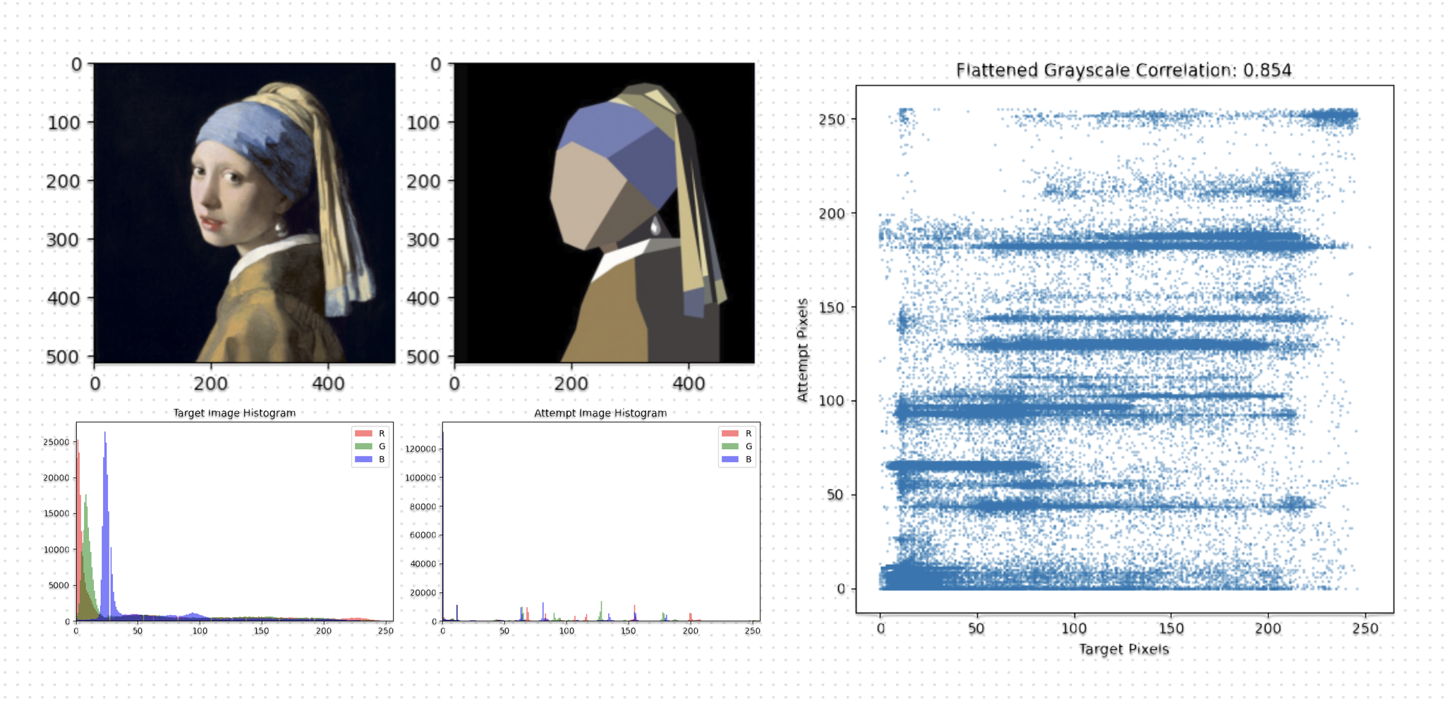
Histogram difference is global and ignores pixel order and correlation checks linear relationship between pixel values. To find the image similarity using histogram difference, we have to compare the frequency distributions of pixel intensities or colors between two images, typically by computing the sum of absolute differences across histogram bins. Lower histogram difference values indicate greater similarity in overall color or intensity distribution. Then we convert both images to grayscale, flattening them into one-dimensional arrays, and calculating the Pearson correlation coefficient between these arrays. A correlation value closer to 1 signifies high similarity in pixel intensity patterns, even if spatial positions differ.

That's why it wasn't enough, it just tells you if you have used same colors with the same brightness and contrast or not. I needed a method that considers the structure and the "Actual" similarity...

‍

Structural and Perceptual Metrics

These metrics refer to a family of image similarity measures that go beyond simple pixel-wise comparisons by modeling how humans perceive visual quality and fidelity. They evaluate aspects like luminance (brightness), contrast, structure (spatial relationships), and information preservation, aiming to align with human visual perception instead of just mathematical differences. For these metric i used SEWAR library, which offers the following metrics:

• SSIM (Structural Similarity Index): Measures luminance, contrast, and structure similarity (closer to human perception)
• VIFP (Visual Information Fidelity): Measures information preserved in the image.

They might have some uses in detecting similarities, but it's only on low-level attributes such as luminance, contrast, and structure, overlooking semantic content, contextual meaning, and high-level features. This can be problematic, two images might score highly similar if they share structural elements despite depicting completely different subjects or scenes, or conversely, images of the same object under varying conditions might appear dissimilar. Moreover, these metrics can be tricked by adversarial perturbations that subtly alter pixel values to preserve perceptual scores while changing the image's interpretation, or by transformations like rotations and scalings that maintain statistics but disrupt spatial relationships beyond their evaluation scope.

So I needed something that detects similar features and detail of the the photos...

‍

Keypoint Matching

These techniques offer a significant advancement over structural and perceptual metrics by focusing on local features that are invariant to transformations like rotation, scaling, and affine changes, thereby addressing the limitations of metrics that can be fooled by spatial rearrangements or adversarial perturbations. These methods detect and match distinctive points based on gradients or descriptors, providing a more robust assessment of similarity that considers semantic content and object-level correspondences rather than just low-level statistics, making them better suited for tasks requiring invariance to viewpoint changes. These are the main methods i have tried:

• ORB (Oriented FAST and Rotated BRIEF): Fast binary descriptor for keypoint matching.

• SIFT (Scale-Invariant Feature Transform): Robust, scale and rotation-invariant keypoint detector.

Then I used FLANN  Algorithm to match keypoints between images, and here are the results:

‍

‍

To measure similarity using keypoint matching, first we need to detect keypoints and compute descriptors (I tried ORB and SIFT) for both images. Then, match descriptors using a matcher like FLANN which stands fo Fast Library for Approximate Nearest Neighbors (We could also try Brute Force Matching), often applying a ratio test to filter good matches. Similarity is quantified by the number of good matches relative to the total keypoints or a minimum threshold (for example, if the match ratio exceeds 0.1-0.2, the images are considered similar, indicating shared features despite transformations).

I know it looks really cool, but it still has flaws, including sensitivity to occlusions, low-texture regions where few keypoints are detected, and potential mismatches in cluttered scenes. Also, it may not capture global context or subtle differences in color and illumination, and computational complexity can be high for real-time applications.

These methods are used for similarity, but the usage is different, it's more useful to detect clones, not differences, so i decided to completely move to another technique that matches and compares the entire image and highlights the differences...

‍

Pixel wise Error Metrics

These metrics compute direct differences between corresponding pixels. It was not abad idea at first, because in applications requiring speed and simplicity, such as realtime quality checks or when images are pre-aligned and transformations are minimal, pixel wise metrics provide fast, interpretable results without the computational overhead of feature detection and matching. They are also more straightforward to implement and debug, making them suitable for baseline comparisons or when semantic invariance is not needed. These are the main metrics i tried in this family:

• MSE (Mean Squared Error): Average squared difference per pixel (lower is better)
• RMSE (Root Mean Squared Error): Square root of MSE (interpretable in original pixel units)
• PSNR (Peak Signal-to-Noise Ratio): Ratio of max signal to noise (higher is better)

‍

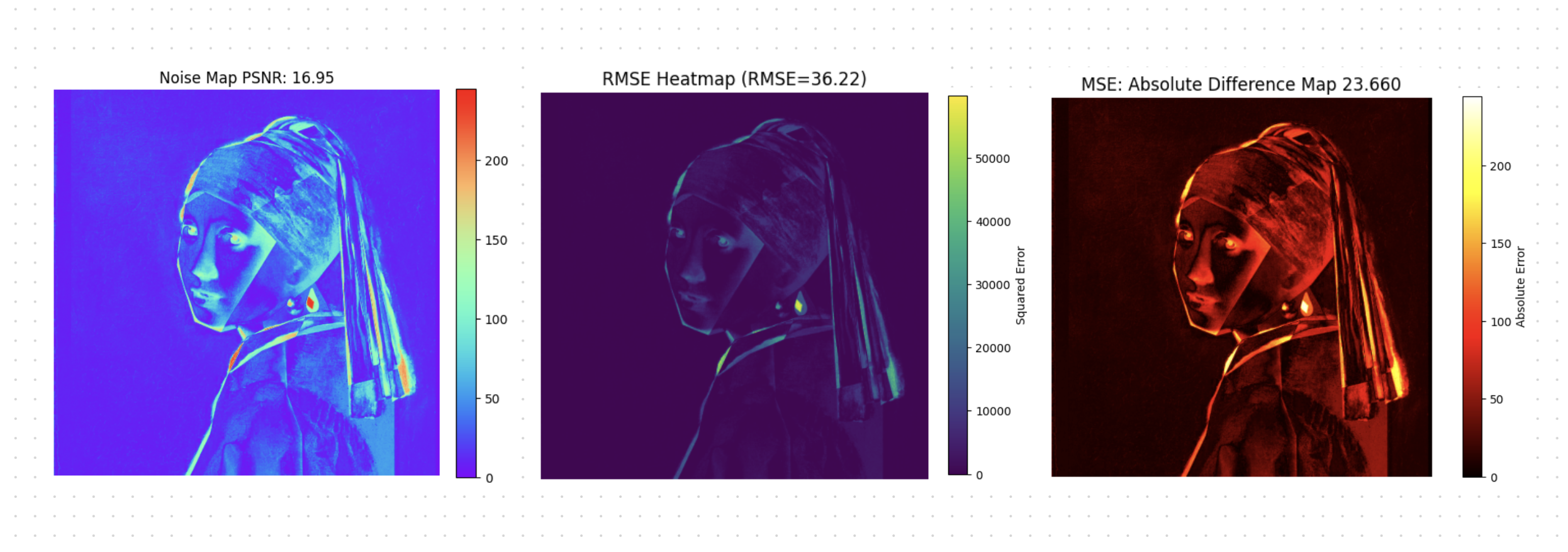
Again, it looks promising, because it clearly highlights the parts of the image that are different, so it gives you an error to subtract from the full score, but there is a HUGE issue, they are highly sensitive to spatial misalignments, lighting variations, and transformations like rotation or scaling. Means they failing when images are not perfectly aligned or have undergone geometric changes, leading to inflated error values even for visually similar images.

‍

Why Classical Computer Vision was not working?

I tried different combinations of these techniques, even created an aggregated system that gives a weight to each metric and calculates the average score, but none of my attempts were good enough. Each metric has different ranges and statistical meanings. For example MSE could be in thousands while the other one is between 0 and 1. I tried to normalize them with arbitrary constants (like subtracting from 1e16) which completely broke interpretability and made the system unstable.

Also I was computing 10 different metrics, many of which were highly correlated. This added computation cost but very little new information. The weighted average at the end was just guessing, because there was no principled way to set the weights. Each new target image or dataset would require manual retuning. The final score had no clear interpretation.

I was convinced that this approach is not working, and I can't do this with the lazy way.The most telling sign that this approach was wrong came when I tried to tune the weights. No matter how I adjusted them, sometimes just a random noise image got higher score than an almost perfect clone.

‍

Then I remembered I know Deep Learning...

While i was doing trialtandherror with the weights, I remembered I can use machine learning to optimize the weights for me. The best metric I had so far was the Pixel Wised Errors, and the only issue was that the system was fundamentally not learning what "similar" meant for this task., and failed with a small misalignment.

If I could train a model that learns the "space of valid variations" of the target image, then candidates that fall within that learned manifold should score well, and candidates that fall outside should score poorly. The reconstruction error of an autoencoder trained on augmented versions of the target would be exactly this measure.

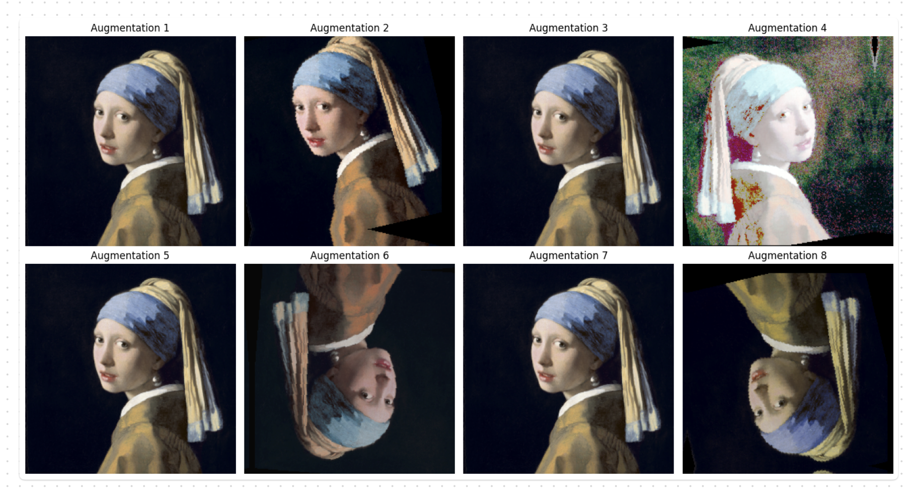
I decided to train a small convolutional autoencoder for each target image. The challenge was that I only had 1 target image, so I needed to generate diverse examples that capture different variations while avoiding overfitting to pixel-perfect identity (we call this method Data Augmentation). I created 250 augmented images from the target image using the following techniques:

• Horizontal and Vertical flip
• Random rotations
• Color jitter (brightness, contrast, saturation, hue)
• Perspective distortion
• Random crops with padding

‍

‍

The Autoencoder Architecture

The architecture I built was simple yet powerful. The encoder starts with the input image at 256x256 pixels and progressively compresses it through four convolutional layers, each with a stride of 2 that halves the spatial dimensions while doubling the number of channels (from 3 initial RGB channels up to 512 in the deepest layer), this downsampling transforms the image from a detailed picture into a compact 16x16 feature map, with batch normalization and ReLU activations ensuring stable, efficient learning along the way. It's like distilling the visual essence, stripping away the noise to focus on the core structure.

‍

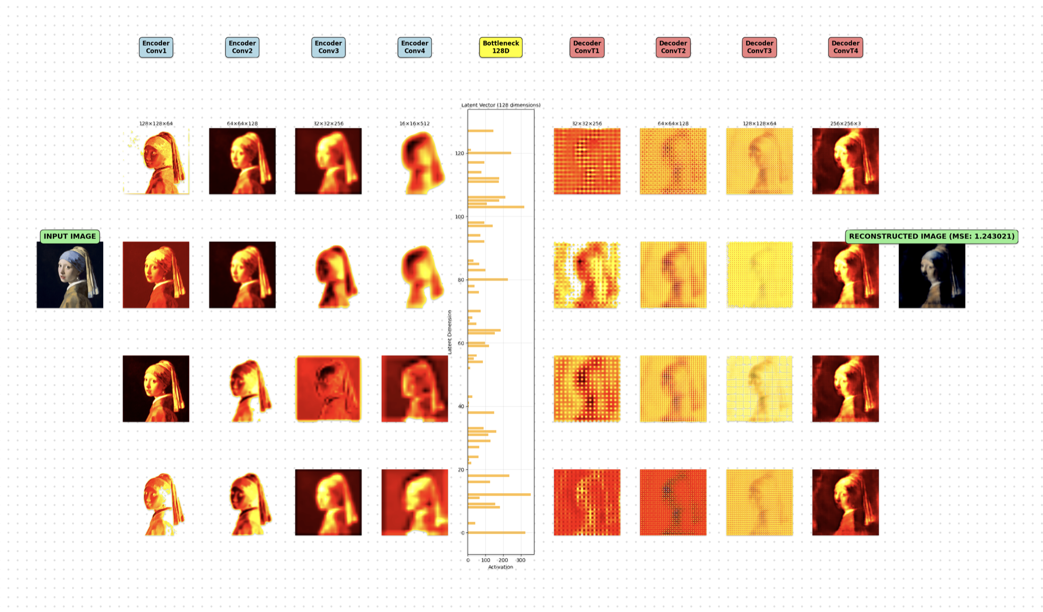
At the middle of the model I added the bottleneck, a deliberate constraint that forces the network to make tough choices. Here, the spatial features are flattened and squeezed through a dense layer into a mere 128-dimensional latent vector. This compression is actually intentional, it's not about preserving every pixel but about capturing the semantic structure that defines the target image. I could have opted for a U-Net with skip connections, which would reconstruct images almost perfectly, but that would defeat the purpose. By funneling everything through this narrow bottleneck, the model learns to prioritize what's actually important, discarding small details that don't contribute to the image's identity.

Finally the decoder mirrors the encoder's path, but in reverse. It starts by expanding the 128-dimensional vector back into spatial dimensions, then uses four transpose convolutional layers to upsample from 16x16 back to the original 256x256 resolution. The final layer outputs a reconstructed RGB image, ready for comparison. The loss function is straightforward: the same pixel wise mean squared error between the input and its reconstruction. But the magic isn't in the loss itself this time, it's in what the model learns from the training data, how it internalizes the variations that are acceptable for this particular target.

What makes this bottleneck so crucial is its role in discriminative power. Images that share the target's essential structure will reconstruct with low error, while those that deviate significantly will struggle. The stride based downsampling ensures the model sees global patterns at a 16x downsampling level, encouraging it to learn overarching structure rather than memorizing local pixels. Batch normalization and ReLU keep training stable and fast, and the model's modest size (relative to today's giant models) prevents it from overfitting to pixel perfect replicas, instead fostering meaningful, generalizable embeddings.

‍

Training the Model and Scoring Submissions

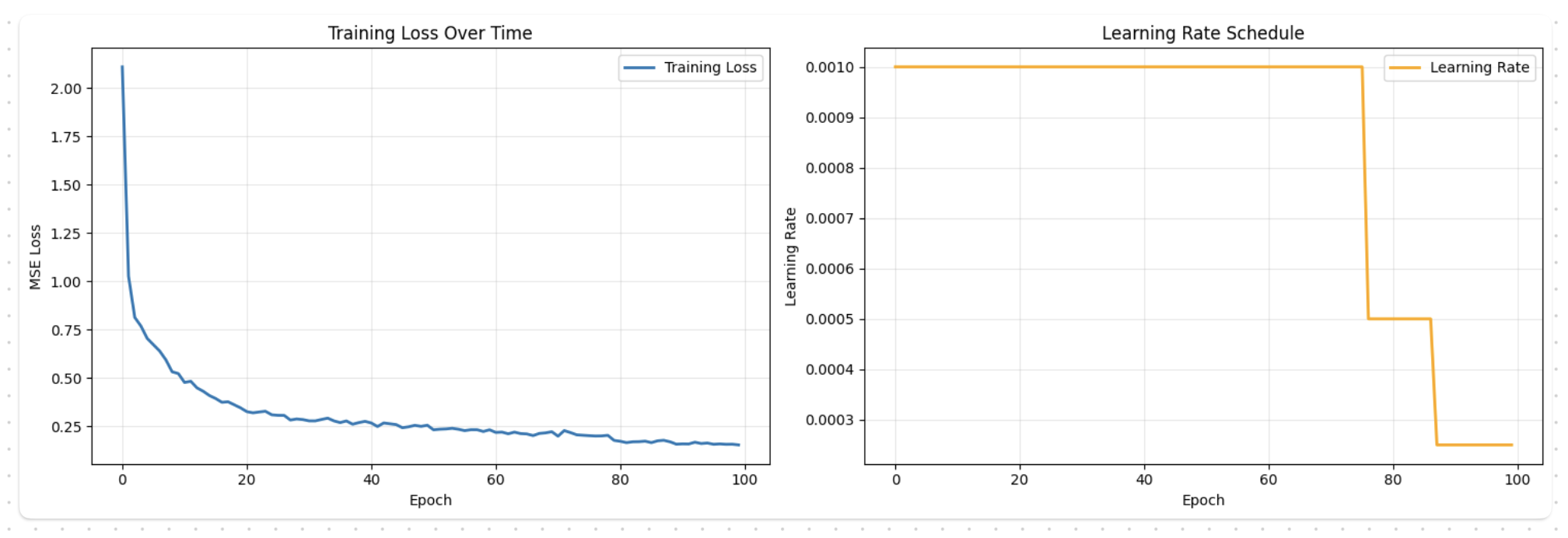
Training this autoencoder was super easy, much better than the complicated weighting schemes I had wrestled with earlier. I used mean squared error as the loss, paired with an Adam optimizer that included weight decay to prevent overfitting. A plateau scheduler adjusted the learning rate based on validation performance, and I saved the best checkpoint to ensure I captured the model's peak understanding of the target (Basically every best practice technique for deep learning)

For each target image, I trained on 250 augmented samples, and it ran for 100 epochs, but thanks to Metal Performance Shaders on my Mac (M1), it completed in just a few minutes, a testament to the model's efficiency.

‍

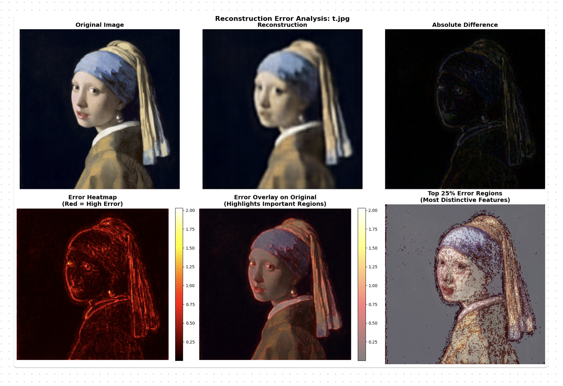
Once trained, scoring a candidate image became elegantly simple. I'd preprocess it to match the training setup (resizing and normalizing) then feed it through the autoencoder. The mean squared error between the original and reconstructed image served as the similarity score: lower error meant higher similarity to the target. This approach was not only accurate but interpretable, I could visualize the reconstruction and generate per pixel error heatmaps to pinpoint exactly where the model detected discrepancies, turning the scoring process into a transparent dialogue between machine and human perception. Here is the same attempt we worked on in previous methods:

‍

‍

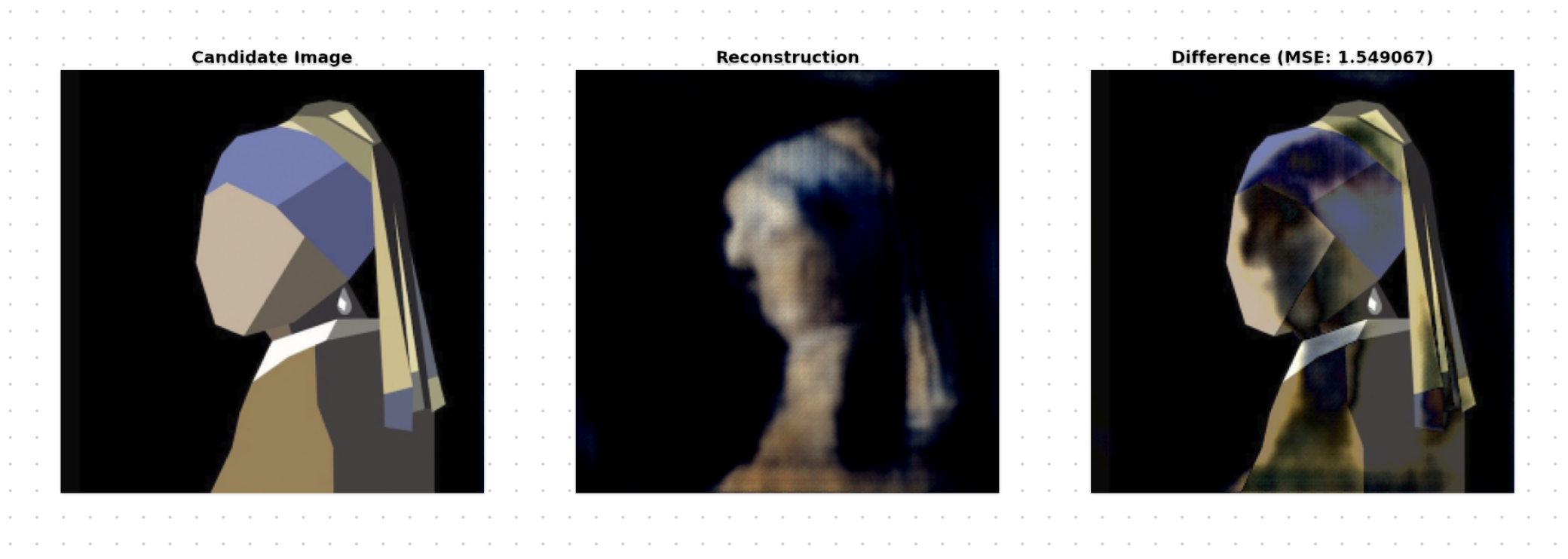
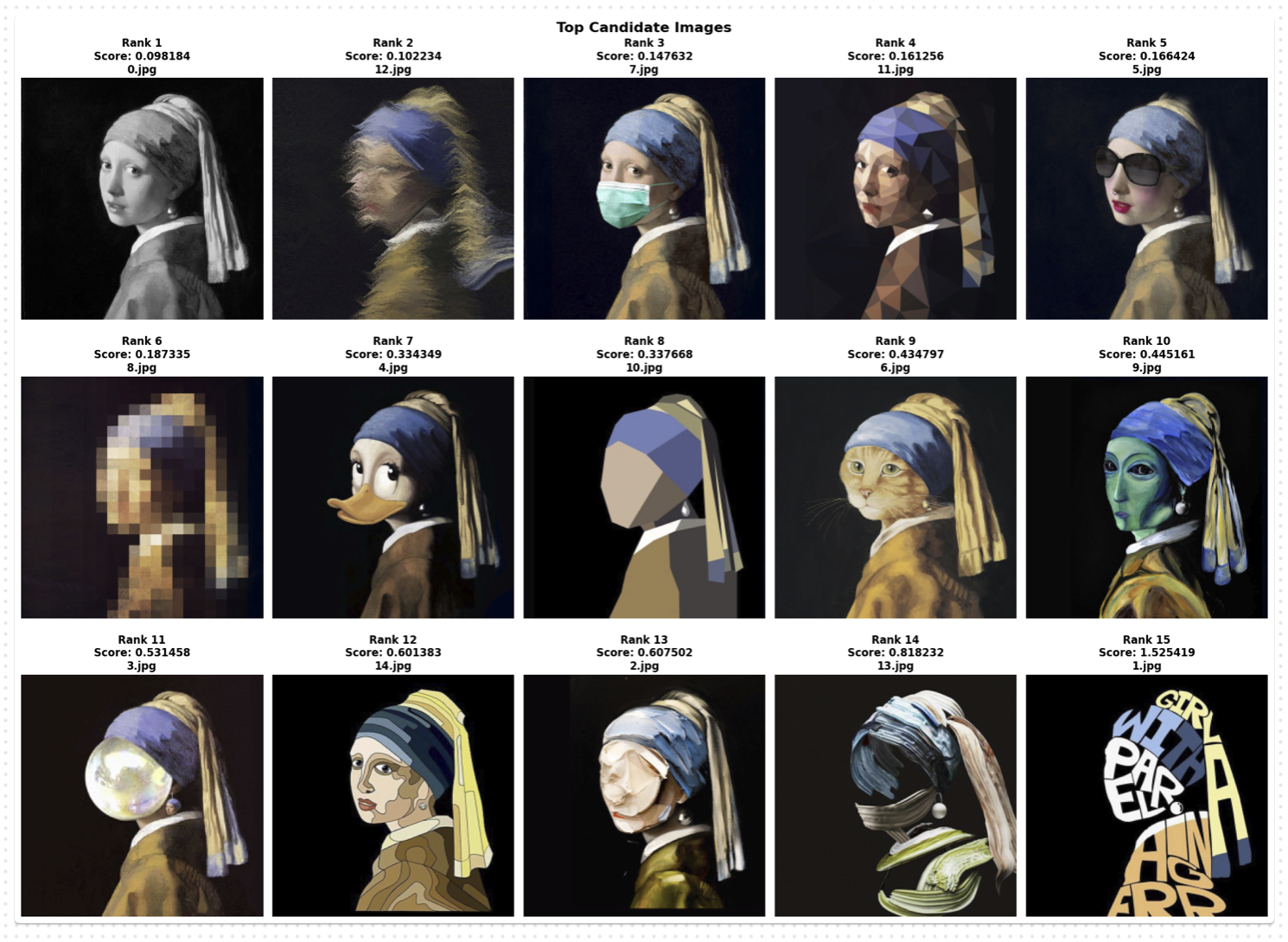
The beauty of this system showed when I tested it on the full set of candidate images, the same meme variations I'd used to challenge the classical methods. The autoencoder didn't just rank them, it understood them. Images that captured the essence of the Girl with a Pearl Earring scored high, while those that strayed too far into parody or irrelevance fell by the wayside. And with the error heatmaps, I could see the model's reasoning laid bare, highlighting unexpected regions and confirming that the scoring aligned with human intuition.

‍

‍

Running the model across all candidates revealed a clear hierarchy of similarity, one that felt natural and fair. The top submissions were those that balanced fidelity to the original with creative interpretation, while the outliers were penalized appropriately. This wasn't just a technical victory, it was a validation of the approach, proving that by training a model to learn the target's manifold, I could create a scoring system that was both robust and human-like in its judgments.

‍